ACAM_64 produces real-time moving images showing sound sources in its field of view. It can be used to find, measure, track and record sources of sound.
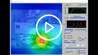
Demonstrates the resolution and response time of ACAM_64
Finger Snap
Demonstrates the directivity of the acoustic beamformer
Crickets Directivity
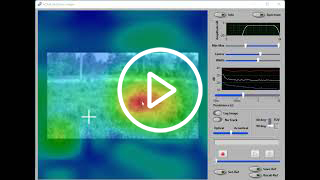
Demonstrates the tracking ability of ACAM_64
Two Cars
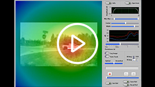
Demonstrates the tracking ability of ACAM_64
Single Truck
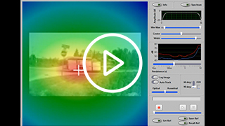
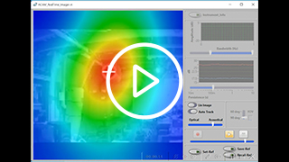
Demonstrates the playback function of a previously recorded movie
HVAC
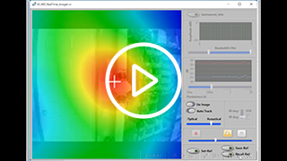
Demonstrates the playback function of a previously recorded movie
Gaz Extractor
Tablet and Tablet-mount are not included with the ACAM_64.
Theory of Operation
An acoustic camera produces an image where the intensity of each pixel represents the amplitude of acoustic waves coming from the corresponding direction. This is akin to an optical camera producing an image where each pixel represents the intensity of light coming from the corresponding direction.
For an optical camera, the lens focuses light coming from a certain direction to the corresponding pixel on the sensor. Each pixel in the image represents the intensity of light coming from a specific azimuth (angle in the horizontal plane) and elevation (angle in the vertical plane). The lens does this by slowing and delaying the light waves hitting the lens by precisely the right amount, so that all waves coming from a certain direction arrive in phase in the focal plane at the position of the corresponding pixel.
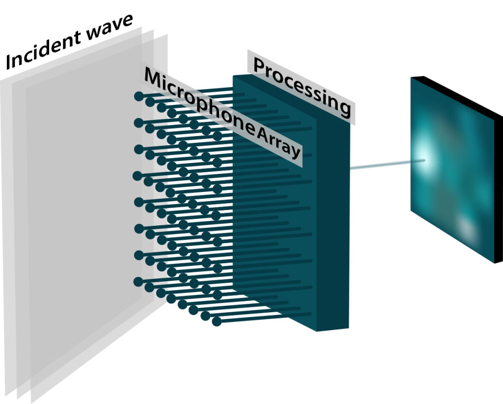
An acoustic camera does much the same thing, except that the work of the lens is replaced by a digital computational engine that processes signals captured by an array of microphones (see Figure 1).
An array of microphones captures the sound waves hitting the array from many different directions. For every pixel, a massively parallel digital processing engine applies specific delays, and sums the signals from every microphone, so that the signals from a specific angle of incidence (azimuth and elevation) arrive in phase. Figure 1 shows that process for a specific pixel. Note that for every arrow from the microphone array, a different delay must be applied, corresponding to the specific angle of incidence and the corresponding pixel. In the simplest implementation, the intensity of the pixel is calculated as the energy of that sum signal, averaged over an adjustable time.
Possible Features
Because the processing is implemented digitally, a few features are possible, some of which are not possible for an optical camera:
The sum signal corresponding to a any pixel position is available and can be streamed out of the processing engine to be listened to. This process is called “beamforming”. The microphone array can be digitally steered to the angle of incidence corresponding to any pixel in the field of view and focus on that source. In addition, since the image shows the azimuth and elevation of the loudest source in the field of view of the camera, the beamformer can follow that “hot-spot” as it moves across the field of view.
A filter can be applied to the processing, such that the camera is only sensitive to certain frequencies. Furthermore, that filter can be adjusted in real-time, while the images are being captured.
The integration time used to calculate the energy of the sum signal for each pixel can be adjusted. This is called the “persistence” of the image and is very similar to the concept of shutter speed for an optical camera. With longer persistence, the resulting image is clearer and less noisy, but successive images blur into each other, making it more difficult to track highly dynamic scenes.
Frequency, Aperture Size and Image Resolution
For an optical camera, as well as for an acoustic camera, the image resolution is a proportional to the ratio of aperture size to wavelength.
For an optical camera the aperture size of the camera (the size of the lens or more generally the light collector) is always very large relative to the wavelengths of interest. This is true even for very small lenses, such as those found in camera phones, where the size of the lens is a few mm, while the wavelengths of interest are in the hundreds of nm (more than 1000 times smaller). For an optical camera, resolution is rarely limited by the size of the aperture.
For an acoustic camera on the other hand, the frequencies of interest often extend to quite low frequencies (long wavelengths). For instance, the wavelength at 100 Hz is 3.4 m. To have a reasonable resolution at such low frequency would require an array of at least 8 to 10 times as large (25 to 30 m wide). This is usually not practical. Therefore for acoustic cameras the resolution is typically poor at lower frequencies and improves as the frequency increases.
Spatial Sampling and Upper Frequency Limit
For an acoustic camera, the maximum frequency is limited by the spatial separation between two adjacent microphones. The half wavelength of the maximum frequency sampled by the microphones must be wider than the distance between two microphones. Otherwise the array is not able to distinguish between sources that are within the field of view, and sources that are outside, leading to artifacts such as phantom images.
For ACAM_64, the distance between microphones is 23mm, so that frequencies up to 7.5 kHz can be imaged properly. In practice the array is sampled at 16 kHz, with a Nyquist frequency of 8 kHz. The anti-aliasing filters in the camera ensure that the signal energy is low above 7.5 kHz.
Field of View (FOV)
The field of view of a camera represents the number of degrees that the camera can see (that are represented in the image) in the horizontal plane (azimuth) and vertical plane (elevation).
For ACAM_64, the field of view is the same in azimuth and elevation (the image is square). There are two possible settings:
90 degrees (-45 degrees to +45 degrees from left to right and from bottom to top)
60 degrees (-30 degrees to +30 degrees from left to right and from bottom to top)
Description
ACAM_64 is an 8×8 microphone array, and real-time beamformer. It can build a 32×32 pixel image of sound sources in real-time, with adjustable frequency response within 20 Hz to 8 kHz.
Its massively parallel beamforming DSP allows the instrument to build each pixel concurrently with no missed sample.
The instrument can be controlled, and the images can be retrieved using an open protocol based on virtual Com port. That open protocol can be used on any platform that has a generic USB CDC driver. That includes Windows, Linux and Mac-OS.
The instrument can stream audio to the host platform through a USB-Audio interface. Through that interface the instrument is seen by the host as a USB microphone. That audio signal is the output of the beamformer and can be steered digitally to any azimuth and elevation in the field of view of the camera. Using the provided Windows application, the beamformer can even track any acoustic source in the field of view.
That USB-Audio interface works on any platform that has a generic USB-Audio driver. That includes Windows, Linux and Mac-OS.
A complete Windows application is provided to operate the camera, view and record images of the sound source.
The Acoustic Camera ACAM_64, is a composite USB device that includes multiple interfaces with their own descriptor information. To ensure that all three interfaces worked together properly and could be serviced by the MCU without timing issues, they utilized the Beagle USB 480 Protocol Analyzer in all development phases including testing, debugging, and final validation.
Want to learn more on Features and Specifications of our new Acoustic Camera, ACAM_64?